PART I: USING SAS FOR THE PC—AN OVERVIEW

1.0 INTRODUCTION

The statistical package SAS (Statistical Analysis System) is a large computer program specifically designed to do statistical analyses. It is very flexible and powerful, and is very popular among researchers because of these characteristics. SAS allows us to input and manipulate data, and to perform many of the calculations necessary for a wide variety of statistical analyses.

This guide is an extremely brief introduction to the functions of the SAS System, and is designed specifically to help you use this statistical package to complete your coursework in your HUGSE statistics courses. Therefore, in many cases, there are different ways to accomplish a task in SAS. For example, there are literally dozens of ways of completing the task of reading in a data file for analysis. In this book, we will focus on the simplest, most direct method for reading in the types of data files provided to you. Obviously if you encounter other types of data files in your future work, the methods outlined here might not be the most appropriate.

Throughout this guide, you will encounter the following symbol alerting you of helpful tips and shortcuts (ø). We hope you find them useful as you use The SAS System.

2.0 ACCESS to the SAS System

All of the computers in the HGSE computer lab are equipped with PC SAS. This then, is the easiest and cheapest way to gain access to PC SAS. You may purchase a license for PC SAS if you wish to have it on your home computer—see your S-030 syllabus for more information about this option.

3.0 USING SAS

3.1 Starting SAS and Understanding the Screen

Start the SAS System by first clicking once on the Start button, then clicking once on the program button, followed by clicking once on the program group labeled The SAS System, and finally clicking on The SAS System for V8. Upon opening the program, 3 important windows are automatically opened: the Log, the Enhanced Editor, and the Output. The Log and Enhanced Editor are immediately visible, while the Output window is underneath these windows. Each of these components will be explained in much more detail in the coming sections. On the left-hand side of the screen, there is also a window labeled Explorer. This window can be helpful for file management, but we will not describe it here, as it is not directly related to conducting statistical analyses with SAS.

The Enhanced Editor: When the SAS System opens, the default active window is the Enhanced Editor window. You will know that the Enhanced Editor is the active window because it has a dark blue stripe at the top. The Log window has a gray stripe, indicating that it is inactive. The Enhanced Editor window is where you will write programs that you wish to run on the SAS System. These programs will consist of a series of SAS commands that will read in and manipulate data, as well as perform statistical analyses. Once a program has been written and saved, the program name will appear next to the word Editor at the top of the window (replacing the word “Untitled1”). You may then recall the program at any time to edit it and rerun it.

Also notice the small blue “+” in the corner of the little notebook page at the top of the editor. This indicates that you are working with the Enhanced Editor as opposed to the Program Editor. The Enhanced Editor color-codes your program for you as you type (see below). This feature is invaluable! We highly recommend that you use the Enhanced Editor when creating your programs. It will help you avoid being frustrated by small syntax errors that can prevent your programs from running properly. This feature is not available on the mainframe version of SAS that has been used in HUGSE statistics courses in the past, to the dismay of many students before you!

The Log: The Log window opens directly above the Editor. Once you have run a SAS program, important information is automatically displayed in the log window. This window will contain a running list of all of the SAS commands that have been executed, and will include information about whether any errors occurred during the program’s execution. For example, when reading in a data file, the Log window will display how many records were read in, and how many variables were contained in each record, allowing you to confirm that the data were read in correctly. It is always a good idea to inspect the Log window to confirm that your program ran as expected before looking at the results of your analyses.

The Output: As one might expect, when SAS successfully runs a program file, the results of your analyses are displayed in the Output window. As you submit future programs, the results will be added to the end of the Output, giving you a running history of the results from your SAS session. You can, of course, clear the contents of the Output window, or any other active window, at any time (which is often useful if there were errors in your program that make the results invalid).

ø To clear the contents of the active window, press CNTL-E. This shortcut is quite useful, especially if you run a program that produced incorrect output. You’ll want to clear the output window of the incorrect output, and clear the log of the error messages.

3.2 Writing SAS Programs: General Guidelines

Every SAS program you will write has (at least) two parts:

· A DATA step, which reads the data from the raw data file into the program and does whatever variable construction you would like; and

· A PROC section, which performs the statistical analyses you have selected.

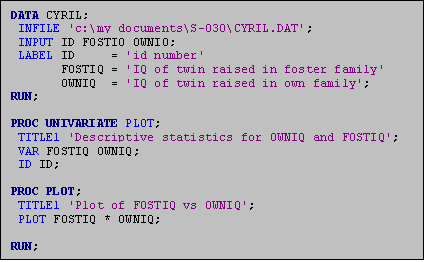Examine the program given below. The DATA statement signals the start of the data step. The word DATA is required, and should be followed by a name you choose for the temporary data set SAS creates and uses as your program runs. In this example, the temporary data set is named CYRIL. The INFILE statement gives SAS the name and physical location of the raw data file that contains the data you wish to use. In this example, there is a raw data file named CYRIL.DAT in the S-030 folder in My Documents. If the file were in another location, this statement would be edited to reflect the physical location of the file. The INPUT statement lists the variables in the data set in the order in which they appear, separated by a space. Be sure to include ALL of the variable names in the EXACT order in which they appear in the raw data file (even if you do not plan to use all of the variables in your analysis). The LABEL statement, (which is three lines, ending in one semi-colon), is written that way because while it is all one statement, it is easier to keep track of the labels if you give each one its own line. This statement tells the computer to label the three variables as specified. The DATA Step ends with the command RUN followed by a semi-colon. This signals to SAS that it should run those commands before proceeding on to the analysis section of the program.

Following the DATA step is a series of procedures (or PROC’s) that perform the desired statistical analyses. The above example has two procedures: the first requests univariate (descriptive) statistics for the variables FOSTIQ and OWNIQ, and the second procedure produces a scatterplot of FOSTIQ by OWNIQ. The last command is the RUN command. This line must appear at the end of your program for the program to run properly.

Important Programming Tips:

ø All statements end in a semi-colon;

ø Major commands appear in dark blue, and begin at the left margin;

ø Subcommands appear in royal blue, and are indented;

ø A blank line appears after the DATA step and after each PROC section.

ø Title statements are included both to label the computer’s output and to help you remember what each PROC step was intended to produce. These titles (and all other commands that are within quotation marks) appear in purple on your screen.

While spacing and titles are not crucial (SAS will run the program even if you don’t organize it this way), using these conventions will help you in the future, especially when you are running much longer and more complex programs. In addition, it allows another person (e.g., your S-030 TF!!) to decipher your program much more easily. Therefore, we advise getting in these habits from the beginning!

3.3 Running SAS programs

Once you write a program, first SAVE IT! If you have made changes to a program, an asterisk (*) will appear next to the file name until you save it again, to alert you that there are unsaved changes. Once you’ve saved your program, you must “SUBMIT” it to the SAS System for it to execute your commands. Submit your program by clicking once on the Submit button (which has an icon of a man running on it).

ø You can also SUBMIT a program by pressing the F8 key.

3.4 Examining the Results of Your Analysis

As mentioned above, once a program has been run, information is written to the Log and Output windows. Always examine the contents of the LOG to ensure that your program ran as you expected. Once you are satisfied that no errors have occurred, continue on by looking at the Output window to see the results of your analysis. You may print or save the contents of either of these windows at any time. By convention, the log file is given a .log extension, and the output file is given a .lis extension (which stands for “listing”).

PART II: CREATING SAS DATA SETS

1.1 Raw Data Files

SAS is capable of reading data files created by many different programs, and converting them to SAS data sets. For your statistics classes here at HUGSE, the data files that you will use are raw data files. By that, we mean that the data are simply entered in a text file (sometimes referred to as an ASCII file). In it, the data are organized either by columns (with column numbers) or by being separated by a particular delimiter (usually a space). In either case, the file contains only the data; it does NOT include any variable names, variable or value labels, or any other formatting. These files are the simplest way to store data, and many programs can convert files to this simple format, allowing you to use the programming methods described here to analyze data from a wide variety of sources.

For most of your analyses for statistics classes at HUGSE, we have already typed the data into the computer and placed it in a raw data file. But you too can create data files if you so desire! The most straightforward method for creating a raw data file from scratch is to enter it into any word processing program (Word, Notepad, etc.), using either the column input format or the list input format that were mentioned above. Both methods require that the variables are entered in order, and the records are separated by a return. Depending on the data format you use, the commands that you will use to read in the data set are slightly different, as you will notice below.

Below are 5 records of a data set called JUNK.DAT with data corresponding to different types of junk food. First the data were entered using column input format, and then using list input format.

In the first data set, columns 1-20 were assigned to the variable ITEM, which represents the name of the item. The number of CALORIES is in columns 22-24, PROTEIN is in columns 26-29, FAT in columns 31-34, FAT_PC in 36-37, SODIUM in 39-42 and COST in 44-47. The information contained in column 49 represents the TYPE of food (burger, chicken, fish, potatoes, shakes, breakfast, or specialty). It is coded using a numeric code for each of these categories.

In the second data set, these same variables appear in the same order. However, each time there is a space, SAS knows that it is to put the value in a new variable. To accomplish this, none of the Item names could have spaces, since SAS would interpret this as a sign to move on to the next variable.

In the sections below, we will outline how to read in data sets in both of these formats using a Data Step.

1.2 The Data Step

The DATA step is the part of the SAS program that reads the data from a raw data file and creates a special data file called a SAS data set. To create a SAS data set from a raw data set, you need to create a SAS program with at least the following three SAS statements:

· A DATA statement

· An INFILE statement

· An INPUT statement

Other optional statements that allow you to create new variables, add labels, and execute other functions can be added to the data step. Some of the more frequently used DATA-step options are discussed in Section III of this manual.

The SAS data set created is what is called a working data set and will only last as long as the current SAS session. When you quit SAS, the working data set will be erased, but the raw data file from which it was created will, of course, remain saved and unchanged. To recreate your SAS data set, you must simply rerun the SAS program file that created it.

1.3 The DATA Statement

As mentioned above, to read a raw data file using SAS you need to create a SAS program file (see below). To read our raw data file called JUNK.DAT, we created a SAS program file called JUNK.SAS. These names were assigned to help us remember what the program was for and the data set with which it went. These names do not have to match, and you can assign whatever program names you feel are appropriate for your purposes.

The program begins with a DATA step. The first line of the DATA step is the DATA statement. The DATA statement tells SAS that you would like to create a SAS data set with a specific name (in our example, JUNK). This is a temporary name that you choose; oftentimes it is convenient to use the same name as that of your data file, but it is not necessary to do so.

Data set names must begin with a letter, and must not contain any spaces. SAS can use names that are longer than 8 characters, but we would advise that you keep your names short and meaningful.

1.4 The Infile Statement

The DATA statement is followed by an INFILE statement. The INFILE statement tells the SAS system the physical location of the raw data file. It begins with the subcommand INFILE and is followed by the path and filename of the file containing the raw data. In the above example, our datafile (JUNK.DAT) is located on the desktop of our computer (whose path is C:\WINDOWS\DESKTOP\). The path and file name must be enclosed in single quotation marks.

SAS Version 8.0 can accomodate the long folder names people often use in organizing their files. So, for example, if our file had been located in the My Documents folder, rather than on our desktop, the path and file name would have read C:\My Documents\JUNK.DAT.

ø use the colors to be sure that your program is written correctly! For example, if the word INFILE does not appear in royal blue, you’ve forgotten your semi-colon for the preceeding command!

ø check your log file! If your path and file name are not specified correctly, your log will produce an error that reads “Physical file does not exist.” This will alert you that SAS did not find the file in the location that you specified.

1.5 The Input Statement

The INPUT statement specifies the location of each variable in the raw data set. Input statements begin with the word INPUT, followed by the names of each variable in the data set in the order in which they appear. The program above is written for the data set entered using the column input format, and therefore includes the column numbers where SAS can expect to find the variables. If we were reading in the data set entered using the list input format, we could eliminate these column numbers.

SAS distinguishes between two types of variables: character variables and numeric variables. Character variables contain information that includes a combination of letters, numbers and/or symbols. Numeric variables contain only numbers and conform to certain SAS conventions. Variable names must begin with a letter or underscore (_), and contain no blank spaces. In V8, SAS can accommodate variable names that are longer than 8 characters. However, to make programming easier, we recommend that you keep your variable names as short as possible.

In the program above, the names of the variables and the location of the columns are included. The first variable ITEM takes up columns 1-20. The next variable CALORIES takes up the columns 22-24, and so on. The dollar sign ($) after the variable ITEM indicates that the variable ITEM is a ‘character’ variable. All character variables must be followed by a dollar sign ($).

A RUN statement appears after the INPUT statement. This signals to SAS that this is the end of the DATA step, and that the system can proceed with reading in the data before executing any of the procedures. This statement is not critical, but it will make your programs run better. SAS will continue to use up temporary memory until it encounters a RUN statement. If you try to execute too many commands before giving SAS a RUN statement, it may run out of temporary memory and be unable to continue.

PART III: USING SAS TO ANALYZE DATA

1.0 INTRODUCTION

This section of this manual outlines some of the commonly used SAS procedures. SAS procedures are placed after the SAS data step in your SAS program file. They always begin with a PROC statement followed by the name of the SAS procedure.

We begin by describing two non‑statistical procedures‑‑PROC SORT and PROC PRINT. We then turn to the basic statistical procedures that you will be using for your course work: PROC UNIVARIATE, PROC PLOT, PROC CORR, PROC REG, PROC GLM, PROC TTEST, PROC CHART and PROC FREQ. We conclude by describing data set manipulations and general options for conducting data analyses and improving the quality of your printout.

2.0 PROC SORT

PROC SORT has two main purposes: to arrange the observations in the SAS data set in a specific order (such as alphabetical or increasing numeric order) and to prepare data for a statistical procedure. PROC SORT does not produce any output. If you want a printout of the sorted data, you must include a PROC PRINT in your program.

2.1 Arranging Data in a Specific Order

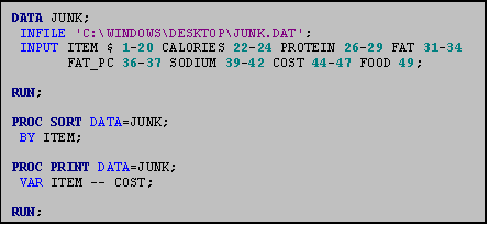Suppose, for example, that you want an alphabetic listing, by ITEM, of the observations in the junk food data set. A PROC SORT statement will sort the data. You need two different statements to run PROC SORT: The PROC SORT statement itself, and a BY statement which specifies the name(s) of the variable(s) by which you want to sort the data.

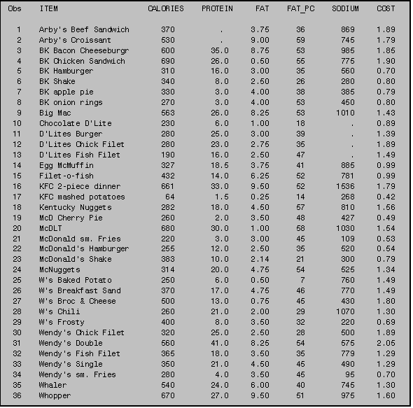
In the program to the right we sort the junk food data set by ITEM. Since ITEM is a character variable, this sort produces an alphabetic listing (as shown in the output file below). Had we sorted by a numeric variable, PROC SORT would produce a rank ordered listing, with the observations in ascending order by the variable we sorted with.

ø The use of the double hyphen (‑‑) indicates to SAS to run the procedure on the two variables listed plus all variables listed sequentially in the input statement between these two variables. Use of the "‑‑" can save lots of typing time, but can be dangerous when working with large data sets with lots of variables because you can mistakenly produce a lot of unneeded output.

2.2 Sorting by More Than One Variable

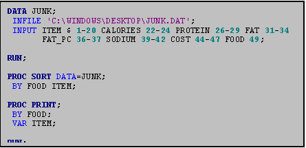On occasion, you may want to sort your data hierarchically by more than one variable. Suppose, for example, that you would like an alphabetical listing of the ITEM variable within each FOOD group. You would sort the data set JUNK by the FOOD variable and then by the ITEM variable. All you must do is sequentially list the several sort variables in the BY statement of the PROC SORT.

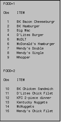
The procedure sorts first by the first BY variable encountered, and then it sorts by the second BY variable within each group of the first BY variable (See program above).

As PROC SORT produces no printed output, you must us a PROC PRINT to obtain the results of your sort. In the example to the left, note that because we only asked for one variable in the PROC PRINT VAR statement, the listing includes only that variable.

2.3 Retaining an Unsorted Version of the Data Set

Sometimes you want to retain an unsorted version of your data, as well as create a sorted version. Why would you want to do this? The reason is consistency. Every time SAS runs a procedure it uses the most recently created data set unless you specify a different data set using the DATA= option on the PROC statement. So unless you indicate otherwise, SAS will not retain the unsorted data set and will use the sorted data set in all subsequent analyses. This may make it difficult to identify specific observations in the data set.

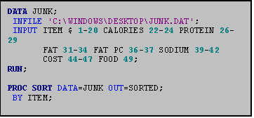To retain the unsorted version, use an OUT= option in the PROC SORT statement. This tells SAS to let the unsorted version remain with its original name and to store the sorted version in a new SAS data set specified by the OUT=option. You can call this new SAS data set anything you would like providing that you follow the data set name conventions specified in PART II Section 1.3. In this example the sorted data set is called SORTED.

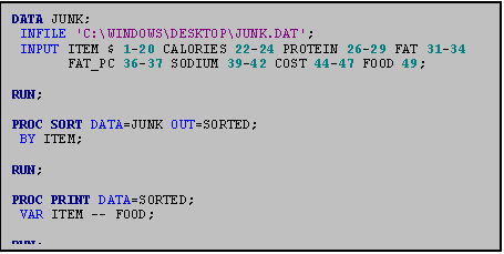
To use the sorted data set in an ensuing procedure, use a DATA= statement, specifying the name you have chosen for your sorted data set. In this case SORTED is specified in the DATA= statement of PROC PRINT. (See Example III: 2.3b). To use the unsorted data set in an ensuing procedure, use a DATA=option identifying the original data set.

2.4 Preparing Data for Ensuing Statistical Procedures

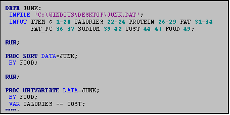
Any SAS procedure that uses a BY statement must be preceded by a PROC SORT. Sort your data by the variable(s) used in the BY statement of the ensuing procedure. For example, in the junkfood data set, if you want to program a PROC UNIVARIATE for each FOOD group you would first sort the data BY FOOD. See Example III:2.4.

3.0 PROC PRINT

PROC PRINT allows you to obtain a printed listing of the contents of data sets. Suppose you wanted to list the data in the junk food data set. To do so, you would invoke PROC PRINT, followed by the names of the variables whose values you would like to print (in a VAR statement). In Example III: 3.0 we print each of the variables in the junk food data set.

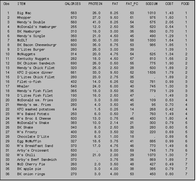
When SAS runs PROC PRINT, it gives you not only the variables you asked for but an additional variable‑‑OBS, which stands for OBServation number. This variable is useful in helping you identify particular cases. (For further details, see Section III: 14.0: Identifying observations by using _N_.)

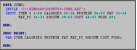ø If you sort data using PROC SORT (see Part III, Section 2.0), SAS assigns observation numbers that correspond to the sorted presentation of the data. Thus, the OBS number associated with a given observation prior to the instigation of the PROC SORT procedure may differ from the number associated with the same observation after sorting. The listing here did not involve any sorting so we see the data as they were entered into the computer. The output generated by the program above appears on the following page.

4.0 DESCRIPTIVE STATISTICS

4.1 PROC MEANS

PROC MEANS computes the sample mean, minimum and maximum values, and standard deviations of all or selected variables in a given data set. Only two commands are required: PROC MEANS (which invokes the procedure) and a VAR statements (which tells SAS which variables to use in the calculations).

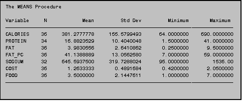In this example, the means from all the numeric variables in the data set JUNK.DAT are displayed. When you do not specify variable names in a VAR statement, SAS will generate statistics on all numeric variables. Be careful: you could get more information than you bargained for.

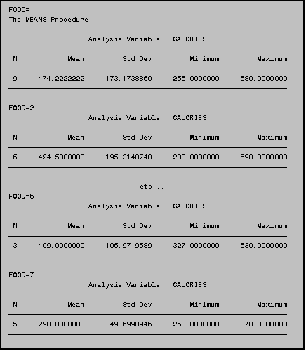
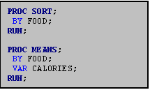You can also use PROC MEANS to obtain group means. For example, supposing you want a list of average calories by food type. In the JUNK.DAT data set the variable FOOD represents various types of food (1=burgers; 2=chicken; 3=fish; 4=potatoes; 5=shakes; 6=breakfast; 7=other). To obtain the means for each of these groups you use a BY statement as in the program to the right, which generated the output below. Remember that the data set must first be sorted according to the BY group, using PROC SORT. For more information on sorting data see Part III, Section 2.0.

4.2 PROC UNIVARIATE

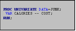
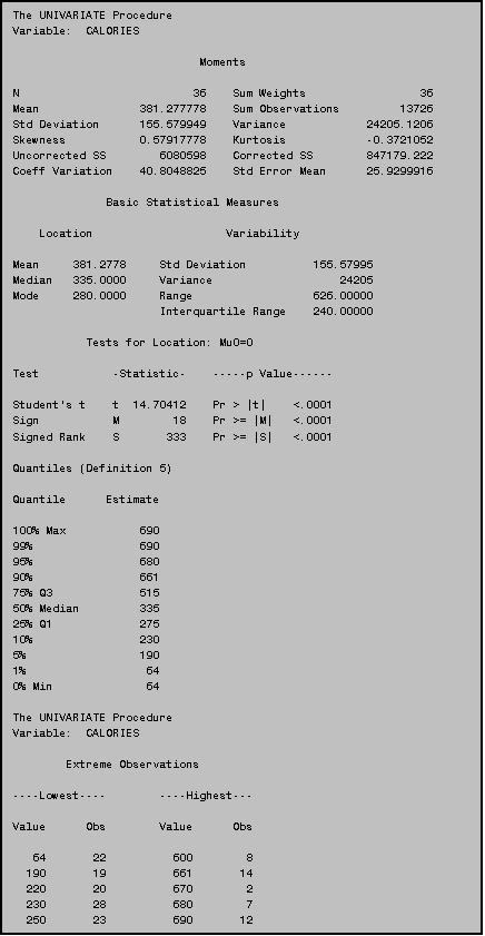
PROC UNIVARIATE generates many useful summary statistics. Its syntax is similar to PROC MEANS‑‑all you do is invoke the procedure with a PROC UNIVARIATE statement, and list the variables to be used in a VAR statement. The program to the right produces univariate statistics on the variables CALORIES PROTEIN FAT FAT_PC SODIUM and COST. Use of the double hyphen (‑‑) tells SAS to run the procedure on the two variables listed plus all variables listed sequentially in the INPUT statement between these two variables. Use of the double hyphen (‑‑) can save lots of typing time, but can be dangerous when working with large data sets with lots of variables.

The first page of the output produced by the program is presented below. Similar output would be produced for each of the five other variables.

ø When the VAR statement is omitted from PROC UNIVARIATE (and other PROC's such as PROC MEANS) SAS will use all the numeric variables in the data set. Although it is tempting to use this typing short‑cut, omitting the VAR statement is not recommended because it may result in generating unneeded output.

4.3 Identifying Observations in PROC UNIVARIATE

In PROC UNIVARIATE, SAS identifies the five highest and five lowest observations in the data set. If you do not provide an identification variable, SAS will use the observation number to identify specific observations as in the example above.

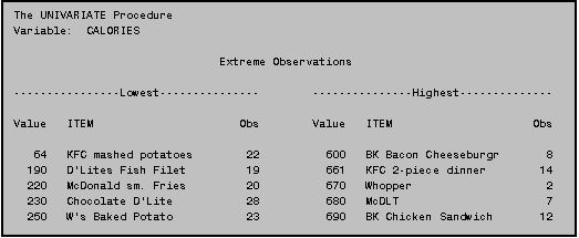
You will often find it handy to have SAS identify the observations using a more meaningful identifier such as an ID number or a name that describes the particular observation. You specify the variable to use in an ID statement. All you do is add the ID statement and follow it by the name of the variable you wish to use as an identifier. In PROC UNIVARIATE, ID statements should be placed after the VAR statement. In the program above, we used the ITEM name as the identifier, so that the PROC UNIVARIATE results indicate the specific items with the five lowest and five highest calorie counts. Using this new program, the “Extreme Observations” section of the output would now look like this:

4.4 Generating Plots in Proc Univariate

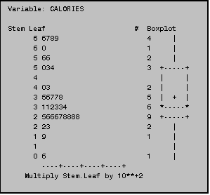In addition to basic univariate statistics such as those provided in the example above, PROC UNIVARIATE will generate stem‑and‑leaf displays and box plots (such as those to the right) when you indicate PLOT in the PROC statement as in the example below:

4.5 Side‑by‑side Schematic Plots in PROC UNIVARIATE

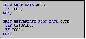If you use PROC UNIVARIATE with the PLOT option and ask for descriptive statistics within a group (using a BY statement) the procedure will produce side‑by‑side schematic plots. Suppose you wanted to create side‑by‑side schematic plots of the calorie counts of the various food groups in the junkfood data set. (Note that the variable FOOD represents various types of food: 1=burgers; 2=chicken; 3=fish; 4=potatoes; 5=shakes; 6=breakfast; 7=other.) You could do so using the program shown at the right.

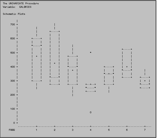In addition to the providing univariate output on the variable CALORIES for each FOOD group, the program above produces side‑by‑side schematic plots as shown below:

NOTE: Before using a BY statement, the data set must first be sorted according to the BY group, using PROC SORT.

5.0 PROC PLOT

5.1 Basic Plots

PROC PLOT generates plots of one variable against the other on the Y (vertical) and X (horizontal) axes. Suppose, for example, that you would like to look at the relationship between COST (Y) and CALORIES (X). The simplest syntax for PROC PLOT is to invoke the procedure, and then use a PLOT statement to ask for the plots of your choice. The syntax on the PLOT statement is Y*X.

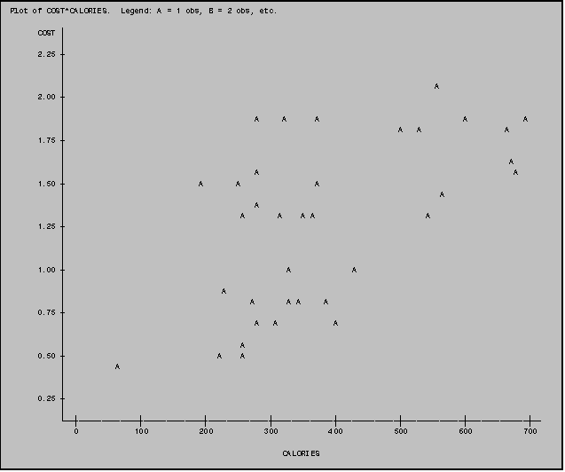
5.2 Designating the Plotting Symbol

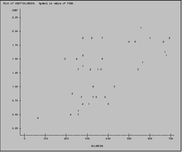
Unless otherwise specified, SAS uses letters of the alphabet as plotting symbols (where 'A' represents 1 observation, 'B' represents 2 observations, etc.). PROC PLOT permits you to specify a different symbol of your choice. Suppose, for example, that you would like to look at the relationship between COST and CALORIES coding the data points by the FOOD variable. You designate the variable FOOD as a plotting symbol by adding an '=' sign after the second (X) variable (CALORIES) and then listing the variable to be used as the plotting symbol (FOOD).

In the plot below the numbers on the plot refer to the value of FOOD for each observation (1=BURGERS; 2=CHICKEN; 3=FISH; 4=POTATOES; 5=SHAKES; 6=BREAKFAST; 7=OTHER). Designating the plotting symbol in this manner can help you identify patterns associated with the various FOOD groups.

NOTE: You can also use a character value (such as the ITEM variable) as a plotting symbol. When this is done the first letter of the character variable is used as a plotting symbol. This can make it easier for you to identify specific observation points.

5.3 Plotting Vertical or Horizontal Reference Lines

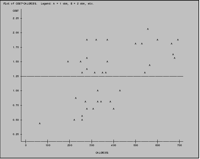
You may sometimes find it helpful to include a reference line on a plot. To do so, you use either the VREF= option to specify one or more vertical references or the HREF= option to specify one or more horizontal references. You use the VREF= and/or HREF= in the PLOT statement after a back‑slash (/) which is placed after the last variable to be plotted.

Suppose, for example that you would like to indicate the mean of the variable COST on your plot of COST by CALORIES. (The mean cost is $1.26.) You would add the VREF option after the PLOT statement as indicated in Example III: 5.3.

NOTE: A vertical reference set to zero (0) is commonly used when plotting residuals (/VREF=0;)

5.4 Multiple Plots

5.4.1 Producing More Than One Plot

PROC PLOT includes a "shortcut" syntax that enables you to produce several different plots within the same PLOT statement. If, for example, you wanted to produce separate plots of your outcome variable (COST) against several predictors (CALORIES, PROTEIN and SODIUM) you could do so using the syntax in Example 5.4.1a. Note that the program in Example 5.4.1a produces the same output as the program in Example 5.4.1b. The program in Example 5.4.1a is a helpful time saver.

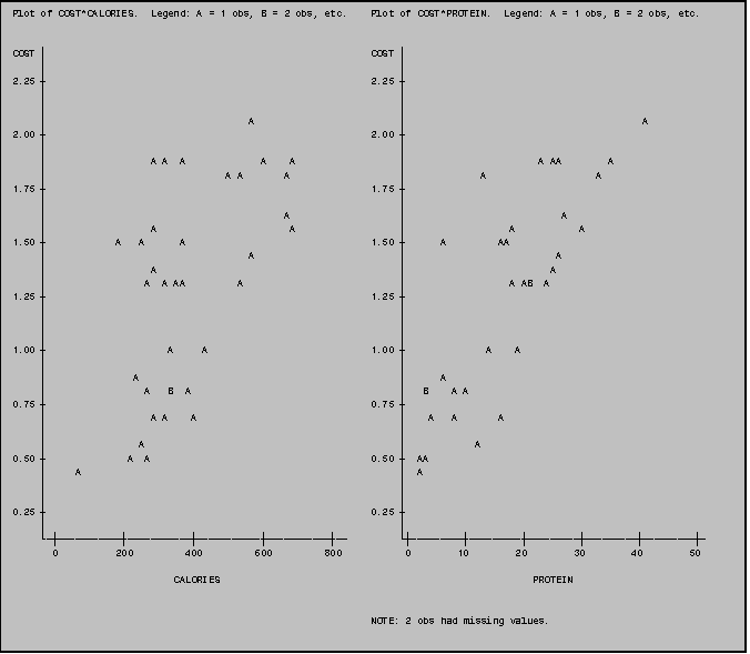
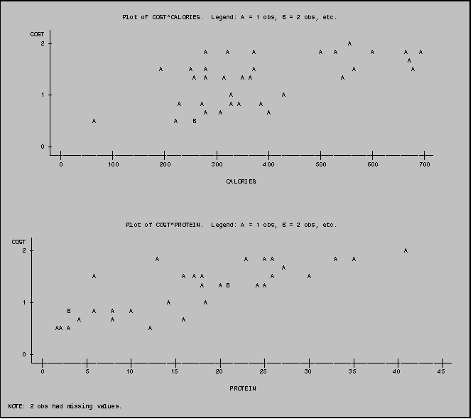
5.4.2 Plotting More than One Plot On a Single Page

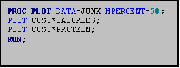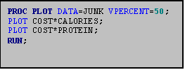
The HPERCENT and VPERCENT options can be used to plot more than one plot on a single page. These options can be helpful when you would like to compare several plots. You add the HPERCENT or VPERCENT option in the PROC PLOT statement. If you would like, for example, two plots placed side‑by‑side on a single page, set the horizontal percent option to 50% by including HPERCENT=50 in your PROC PLOT statement. (See sample program). For three plots use 33; for four, 25 and so on. Similarly, if you would like two plots placed one above the other on a single page, set the vertical percent option to 50% by including VPERCENT=50 in your PROC PLOT statement. (See sample program) For additional plots use the appropriate percentage (33, 25 etc.) as you would for the HPERCENT option. The output produced by these two procedures is shown on the following two pages.

6.0 PROC CORR

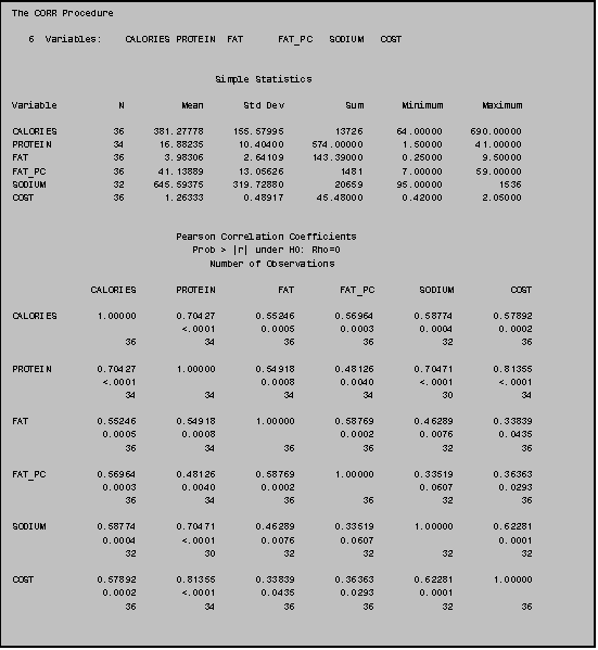
6.1 Simple Correlations

This sample program shows how to use PROC CORR to estimate correlations among the variables CALORIES PROTEIN FAT FAT_PC SODIUM and COST in the junkfood data set. All you do is invoke the procedure and list the variables you want to correlate in a VAR statement.

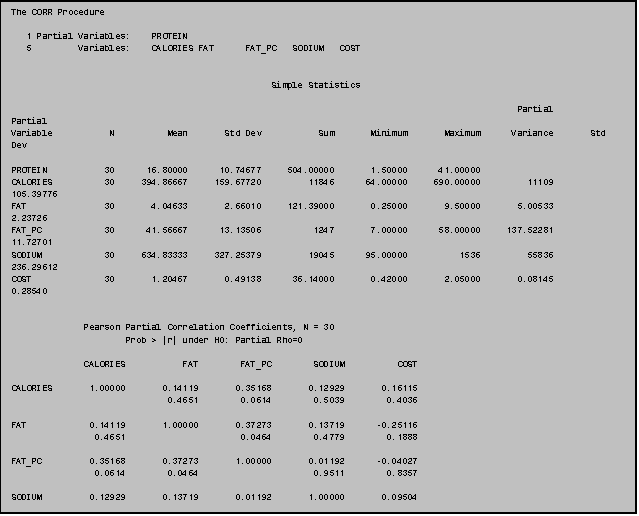
You can also use PROC CORR to estimate partial correlations among variables. You do so by adding the PARTIAL statement after the PROC CORR statement.

7.0 PROC REG

7.1 Simple Linear Regression

PROC REG is a very general regression program used for simple and multiple regression. To fit a simple linear regression model, all you must do is use a MODEL statement in PROC REG that tells the computer what model you would like to fit. Example III: 7.1 illustrates the simplest syntax for a linear regression model.

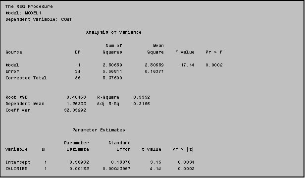
Being an expertly trained researcher, you would also want to inspect the residuals associated with a given regression model. The following sections present three ways to examine residuals:

• listing predicted values (P) and residuals values (R) using the '/P R' option

• examining the distribution of the residuals

• plotting residuals

The techniques for doing these things are described in the following subsections.

7.2 Listing Predicted Values and Residuals

The simplest way to obtain a listing of the predicted values and residuals is to use the /P R option in the MODEL statement in PROC REG (Example III: 7.2).

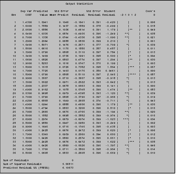
ø If you include an ID statement in your PROC REG, it will identify the observations by OBS number (as in the example above and by this identification variable. SAS inserts this identification variable in a column between Obs and Dep Var. If you wanted, for example, to use the variable ITEM as an identifier the SAS syntax would be as follows:

7.3 Examining Residuals

While adding the /P R option to the MODEL statement in PROC REG will produce a printed listing of the predicted values and residuals for your regression model, it does not include the residuals or predicted values in a SAS data set for further analysis. So a somewhat more complex, but often preferable, way to examine the distribution of residuals or to plot the residuals is to include an OUTPUT statement in your PROC REG procedure.

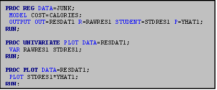When SAS encounters an OUTPUT statement in PROC REG, it creates a new SAS data set, which includes all the old variables as well as all the additional variables you specify, such as raw residuals, studentized residuals and predicted values. To create this new SAS data set you need to place an OUTPUT statement after your MODEL statement. In the OUTPUT statement you name a new SAS data set (using the 'OUT=' option) and the new variables you would like it to contain: the residuals values (using the 'R='option); the studentized residuals (using the 'STUDENT=' option); and the predicted values (using the 'P=' option). In this example, the new data set is called RESDAT1, the raw residual variable is called RAWRES1, the studentized residual variable is called STDRES1 and the predicted values variable is called YHAT1. (You can name the new variables anything you would like providing you follow the variable‑name conventions outlined in PART II section 1.5.)

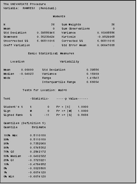
After including an OUTPUT statement in your PROC REG statement you can then analyze your newly created variables (RAWRES1, STDRES1, YHAT1) using PROC UNIVARIATE, PROC PLOT or any other procedure as you would with any other set of variables.

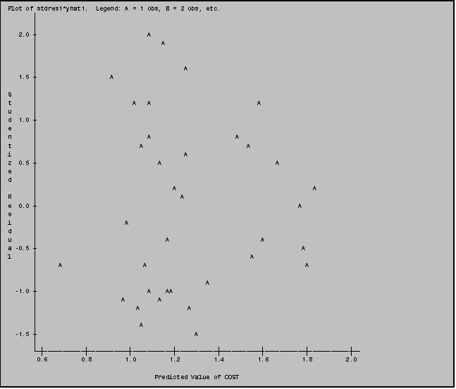
To save space we present only portions of the output from this program: some of the PROC UNIVARIATE results for RAWRES1 and the PLOT of STDRES1 vs. YHAT1.

7.4 Multiple Regression

The syntax for multiple regression resembles that for simple regression. You still use PROC REG; you simply add the additional predictors to the right hand side of the equation in the MODEL statement.

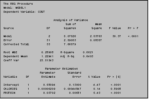
Suppose you wanted to look at the relationship between COST and two predictors, CALORIES and PROTEIN. Simply add the additional variable PROTEIN to the MODEL statement as in the example above.

You may combine the different regression options together in a single program. You may, for example, want to output the residuals from a multiple regression model using an OUTPUT statement (see PART III: 7.3).

7.5 Including an Interaction Term in PROC REG

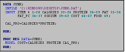To include an interaction term in your regression model first create a new variable, in the data step, representing the cross product term. Then add this new variable to the model statement of PROC REG. If you wanted to test for an interaction between CALORIES and PROTEIN you could use the program to the right. Note the variable representing the interaction term, CAL_PRO, is simply the variable CALORIES and PROTEIN multiplied (*) together.

8.0 PROC GLM

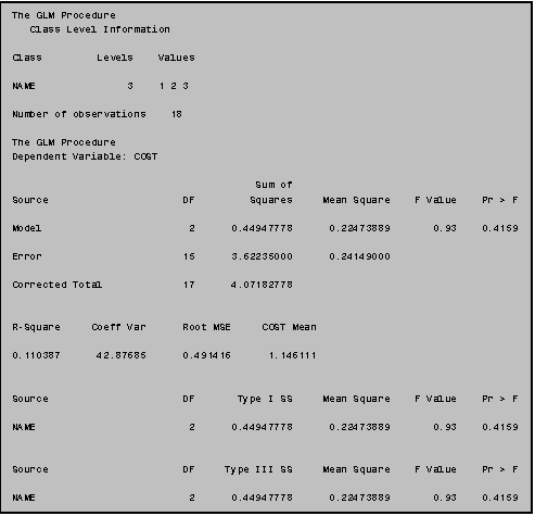
Analysis of variance can be performed using either PROC ANOVA or SAS's General Linear Models procedure (PROC GLM). In this manual we illustrate the PROC GLM procedure.

8.1 Analysis of Variance

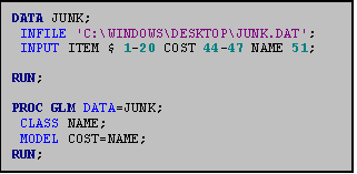For this example, we will use an abbreviated form of the junk food data set. We focus on determining whether the average COST of food varies significantly among three different burger joints (McDonald's, Burger King and Wendy's). The name of the establishment is captured by the variable NAME.

The syntax for PROC GLM is similar to that of PROC REG. You invoke the procedure with the statement PROC GLM and you specify the model to be estimated using a MODEL statement. In PROC GLM, however, if you want to compare group means, you must add a CLASS statement after the PROC statement and before the MODEL statement. In the CLASS statement, you tell SAS that the variable you specify in the MODEL statement is to be treated as a CLASSification variable denoting group membership. The class statement is mandatory. If you omit it, SAS will assume that the variable in the MODEL statement is continuous and it will estimate a regression model using the values of the predictor (if the predictor is numeric) or it will return an error message.

NOTE: If you wanted to conduct a two‑way analysis of variance, all you need to do is add the additional classification variables to the CLASS statement, and modify your MODEL statement appropriately. For a main effects model, you simply list the additional variables in the MODEL statement. If you would also like to investigate interaction effects, you can include these additional terms in the MODEL statement using the *. For example, 'MODEL Y=X1 X2 X1*X2;' would estimate a two‑way analysis of variance model using X1, X2, and their interaction.

8.2 Calculating Sample Means within Groups: Including a MEANS Statement

PROC GLM includes a simple provision for estimating sample means within groups specified by the CLASS variable. All you do is add a MEANS statement after the MODEL statement.

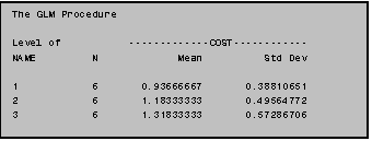
(In addition to the ANOVA output generated in Example III: 8.1 the program in Example III: 8.2a would also generate the output displayed in Example III: 8.2b.)

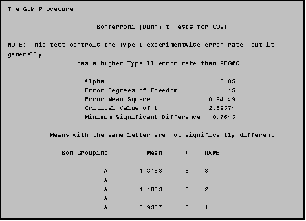
8.3 Multiple Comparison Procedures

To generate multiple comparison tests (such as BONFERRONI t‑tests) you simply add the multiple comparison option (such as / BON LINES) to the MEANS statement. The program to the right produces Bonferroni statistics.

9.0 PROC TTEST

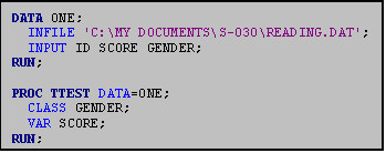If you are only comparing two groups, you can compare their means using a two sample t‑test available through PROC TTEST. Suppose you have tested the reading skills of a sample of eleventh‑grade boys and girls. You are interested in determining whether or not girls score higher than boys on the test. You have two variables, SCORE and GENDER. You could use the program shown here.

10.0 PROC FREQ

10.1 One-Way Frequencies

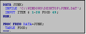PROC FREQ produces a variety of frequency tables. It is particularly useful when you would like to obtain descriptive statistics for categorical variables, either a single variable at a time or more than one variable in relationship to each other. Be sure that the variables you use in PROC FREQ statements are indeed categorical; otherwise you may create reams of output. If the variables are continuous, consider using PROC UNIVARIATE instead.

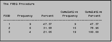PROC FREQ generates several related descriptive statistics. In addition to providing the number of observations for each value of the variable (in the 'frequency' column), the percent of observations for each value is provided in the 'percent' column. The cumulative frequency and cumulative percent is also generated by PROC FREQ.

NOTE: To graphically display frequency statistics use PROC CHART. See Section III: 11.0 for more information.

The program above generates descriptive statistics for the variable FOOD. (Note: For the variable FOOD: 1='burger', 2='chicken', 3='fish', 4='potatoes', 5='shakes', 6='breakfast', and 7='other'). To simplify this example and all ensuing examples in this section we have used a three‑level version of the original seven‑level variable; only burgers (1), chicken (2), and fish (3) have been analyzed.

10.2 Two‑Way Frequencies

When analyzing categorical data, you may want to know how many observations from different categories of one variable are in each category of another variable. You can use PROC FREQ to produce this kind of cross‑tabulation.

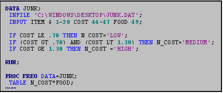
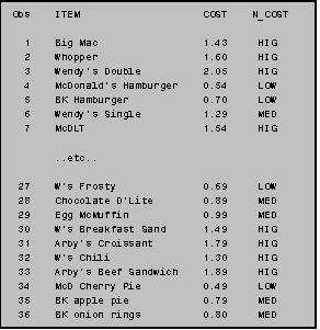
The program at the right generates a two‑way table of the variables FOOD and a newly created variable, N_COST. The variable N_COST is a categorical variable depicting 'low' 'medium' and 'high' values of the continuous variable COST. (For more information on creating this type of variable, see Section III: 12.2.)

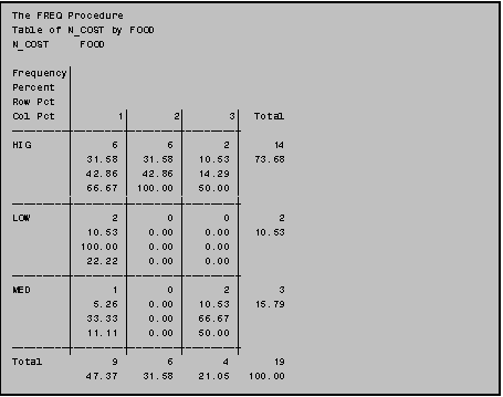
The two‑way frequency tables produced by PROC FREQ (see below) contain a great deal of information. Each cell has four entries: 'frequency', 'percent', 'row pct' and 'col pct'. To understand these entries take, for example, the cell in the top, left‑hand corner. This cell refers to the FOOD=1 category, (burgers) which have a high price (a cost greater than or equal to $1.30). Within this cell, the top entry, the number 6, indicates that, out of the 19 junk foods analyzed, there are 6 burgers with high cost. The entry below the top entry indicates the percent of all junk foods which fall into this cell, that is, 31.58% of the 19 junk foods analyzed are high‑priced burgers. The third entry, 42.86 is the "row percent." This means that of all the 'high' priced junk foods, 42.86% are burgers. Similarly, the final entry, the column percent, indicates that 66.67% of all burgers (that is, foods in the FOOD=1 category) are high‑priced.

NOTE: When PROC FREQ displays alphabetic categories such as the 'high', 'medium' and 'low' designations of the N_COST variable it presents them in alphabetical order. Thus, in this case, 'low' comes before 'medium' and directly after 'high'. If the variable were numeric, its values would have been displayed in numeric order.

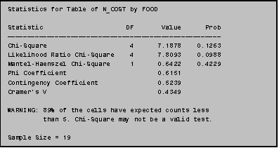
10.3 The Chi‑Square Option on PROC FREQ

You can use PROC FREQ to test the null hypothesis that the variables in the columns and rows of a two‑way table are independent. Computation of the Chi‑square test statistic is one way to test this hypothesis. To generate chi‑square statistics, simply add the '/CHISQ' option to the TABLES statement in PROC FREQ. The output seen below will then be appended to the bottom of the two-way frequency table.

10.4 Other Options for PROC FREQ

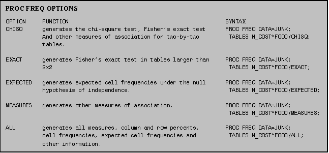In addition to the '/CHISQ' option, PROC FREQ has other useful options that can be added to the TABLES statement. A few of these options are summarized below.

You can use the PROC FREQ options by themselves or with other options. For example, if you would like the expected frequencies included with the chi‑square test you could use the program below.

11.0 PROC CHART

PROC CHART is used to produce graphical displays. It can be used with any type of variable, but is most effective with categorical data. If the variable of interest is continuous, consider using PROC UNIVARIATE or PROC PLOT. In this section we illustrate how to generate three different types of charts: horizontal bar charts, vertical bar charts, and block charts.

11.1 Horizontal Bar Charts

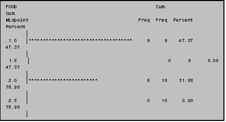
Horizontal bar charts are generated using the HBAR statement in PROC CHART. By default, PROC CHART chooses the number of bars and the midpoint of each bar for the variable you indicate in the HBAR statement. (If you desire, you can specify the intervals, but in Example III: 11.1, the default is used.) The midpoint for each bar is indicated on the vertical axis; the number of observations in each bar (the 'frequency') is indicated on the horizontal axis.

NOTE: To simplify this example and all ensuing examples in this section we have used a three‑level version of the original seven‑level variable FOOD, thus only burgers (FOOD=1), Chicken (FOOD=2), and Fish (FOOD=3) are included.

11.2 The Discrete Option

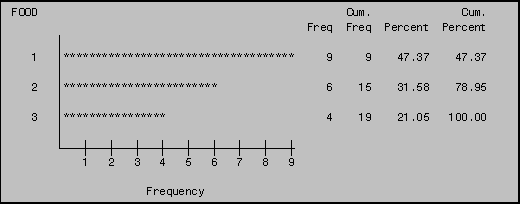
In PROC CHART you can specifiy that a variable has a limited number of values by using the '/DISCRETE' option in the HBAR statement. Instead of indicating midpoints of the variable, SAS will use the discrete numeric values. When producing charts of categorical data be sure to use the discrete option as it improves the readability of the resultant display.

11.3 Creating Charts within Subgroups: The GROUP option

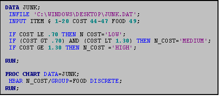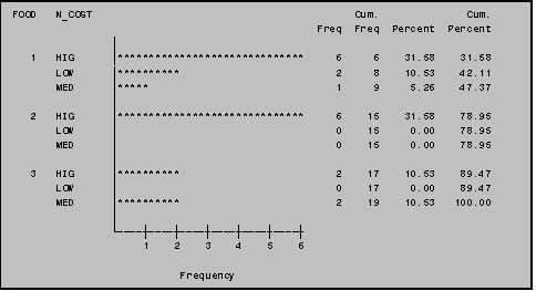
You can also use PROC CHART to display frequencies of one variable by levels of another variable. To do so, use the 'GROUP=' option. Here,.3 levels of the variable FOOD are grouped according to a newly created variable, N_COST. (N_COST denotes 'high', 'medium' and 'low' values of the variable COST.)

NOTE: We include the 'DISCRETE' option in addition to the 'GROUP=' option to improve the readability of the display.

NOTE: Because "N_COST" is an alphabetic variable, the categories are displayed alphabetically, rather than from highest to lowest, or lowest to highest. To avoid this problem we recommend the use of numeric labels.

11.4 Vertical Bar Charts

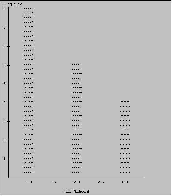
Vertical bar charts are generated using the VBAR statement in PROC CHART. As with the HBAR option, by default PROC CHART chooses the number of bars and the midpoint of each bar for the variable you indicate in the VBAR statement. The midpoint for each bar is indicated on the horizontal axis; the number of observations in each bar (the 'frequency') is indicated on the vertical axis.

As with the HBAR statement, the '/DISCRETE' and 'GROUP=' options can be used with the VBAR statement (see sections III: 11.2 & 11.3).

12.0 MODIFYING SAS DATA SETS

As you learn more about data analysis, you will encounter occasions when you will need to modify your data set. Common modifications include transforming a variable to a different scale; categorizing a continuous variable; and deleting selected observations from a given data set.

12.1 Transforming a Variable to a Different Scale

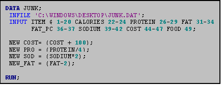Common transformations include power transformations, logarithmic transformations, and square and cube‑root transformations. To transform a variable you: (1) identify a name for the transformed variable using the variable‑naming conventions described in Part II section 1.5; (2) follow the name by an = sign; and (3) type a statement indicating how the variable is to be transformed. For example if you wanted to transform the variable CALORIES to a natural log scale you'd type:

LOGE_CAL = LOG(CALORIES);

In the program above, the variable CALORIES is transformed to a variety of different scales.

NOTE: The new variables are created after the INPUT statement and before any PROC statements. Placement is crucial‑‑you cannot use a new variable until you create it.

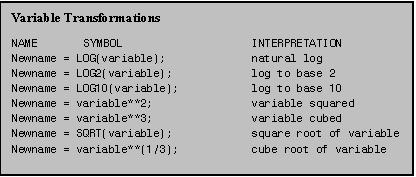SAS has many operators that facilitate variable transformation. Table III: 12.1 indicates the various symbols used to conduct some of the most common ones. Adding, subtracting, multiplying and/or dividing variables are also common ways to modifying variables. Addition is performed using the + sign, subtraction is performed using a ‑ sign; to multiple use a * sign and to divide use a / sign.

NOTE: When arithmetic operators are used, SAS processes the arithmetic operations according to standard mathematical conventions. (You may recall the "Please My Dear Aunt Sally" rule from your 8th‑grade algebra class.) Items in Parentheses are processed first. Multiplication and Division are processed prior to Addition and Subtraction. WHEN IN DOUBT, USE PARENTHESES!

If you are unfamiliar with these conventions, note the following example:

10 + 10/2 and (10 +10)/2

The above arithmetic statements yield two different numbers. In the former, 10 is first divided by 2 and then added to 10 (10 +10/2=15); in the latter, 10 is first added to 10 and then divided by 2 ((10+10)/2=10). These basic mathematic conventions should be kept in mind when creating variables.

12.2 IF/THEN Statements

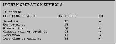Use IF/THEN statements when you would like to specify a condition for carrying out a given operation. You use either any of various symbols or any of various abbreviations to indicate the type of relation you would like SAS to carry out. Table 12.2 summarizes the symbols and abbreviations used in IF/THEN operations.

NOTE: IF/THEN statements should be placed in the DATA step after the INPUT statement.

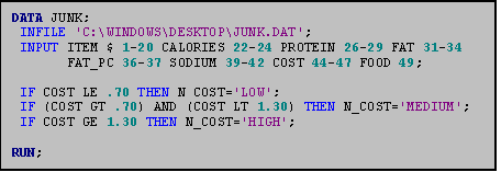Suppose you wanted to group the observations in the junkfood data set according to three categories of COST. You would like to create a new character variable called N_COST (new cost) in which foods costing $1.30 or more are categorized as "high"; those costing between $.70 and $1.30 are categorized as "medium" and those costing $.70 or less are categorized as "low".

NOTE: Because the new variable is a character variable, we use single quotation marks around its values. If we had used numeric labels instead, quotation marks would not have been needed.

12.3 Selecting Observations: Using IF Statements

You can also create datasets which include only specified observations. In a later analysis of the junkfood data set, for example, you might want to limit your analysis to only one kind of FOOD such as burgers. (Remember that in the variable FOOD 1=burgers, 2=chicken, etc.). The use of an IF statement tells SAS to include only those observations for which FOOD is 1.

NOTE: IF statements should be placed in the DATA step after the INPUT statement.

You can also use IF statements to exclude observations from a data set. Suppose you have a data set in which ID is a variable identifying the observation‑number of people in the data set. Suppose, as well, that you would like to conduct an analysis using all subjects except the person whose ID is 20. You could use the following IF statement:

Observations can also be excluded using an IF/THEN statement. The IF/THEN statement at the right is equivalent to the above IF statement.

You can also delete a group of observations using an IF statement. The example on the right deletes those observations whose ID's are equal to 20, 30 and 40.

NOTE: In data sets such as the junk food data set which do not contain a variable identifying observation numbers, you can create a variable ID using one of the SAS "automatic" variables (_N_). For more information see Part III, section 14.1 of this manual.

13.0 MAKING OUTPUT LOOK GOOD

SAS has several options that can be used to make your output easier to read. In this section a few of these options will be discussed. None of these options is required.

13.1 Title Statements

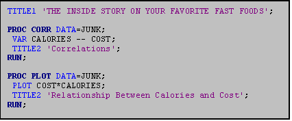The TITLE statement adds a title at the top line of each page of output. You can specify up to 10 lines of titles. Use TITLE1 for the first title line, TITLE2 for the second line, TITLE3 for the third, and so on. Title statements can occur anywhere in your program (that is, before the DATA step, in the DATA step, or in a PROC statement), but every time you use a title the previous title of the same number will be replaced.

ø TITLE statements must be enclosed in single quotes.

The example above illustrates how titles might be used with the junk food data set. Note that the second use of TITLE2 replaces the 'Correlations' title in subsequent output, but TITLE1, 'THE INSIDE STORY ON YOUR FAVORITE FAST FOODS', is printed on every page.

13.2 Label Statements

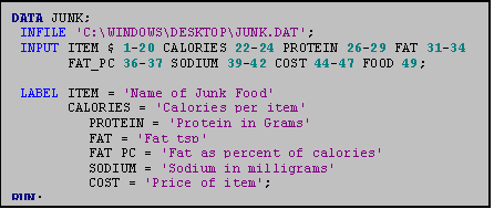Variable labels make it easier to identify variables. You assign variable names in the DATA step using a LABEL statement after the INPUT statement. Note that the label you attach to each variable should be enclosed in single quotes. Additionally, because SAS allows you to label many variables in a single LABEL statement, only the last variable in your list is followed by a semicolon (;).

13.3 PROC FORMAT

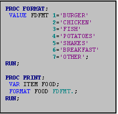While label statements label variables, you may sometimes also want to label values of variables. To assign labels to values of variables, you use PROC FORMAT. In the junk food data set it would be useful to format the variable FOOD.

In PROC FORMAT you create a format by using the VALUE statement. In the VALUE statement you name the format and label each value of the variable. The format name can be anything (as long as it begins with a letter, is eight characters or less and contains no spaces). By convention formats generally end with the 3 letters FMT. In this example we create a format called FDFMT (Food Format). A label (enclosed in single quotes) is assigned to each value of the variable. (In this case 1='burger', 2='chicken' etc.). The last format listed (for a given variable) is followed by a ';'.

In ensuing PROC statements, you invoke the format using the FORMAT command, linking the variable you want to format to the format you created in PROC FORMAT. Note the use of the period (.) after the value name FDFMT. This is necessary SAS syntax. It tells SAS that FDFMT is a format, not a variable.

14.0 Identifying observations with _N_

Several "automatic" variables are available in SAS. One of these is the _N_ variable. This system variable is most helpful when your dataset does not contain an ID or case numbering variable. You can use _N_ to identify the observations. All you do is create a new variable (here called ID) equal to the _N_ variable.

NOTE: Be sure to place the variable‑creation statement (ID=_N_) in the DATA STEP.

PART IV:

TIME SAVING SECRETS EVERYONE WISHED THEY KNEW

A number of time saving "tricks" have been handed down by word of mouth from veteran SAS users to novices over the years. Veterans wished these tricks were in this guide when they were learning how to program SAS for the first time. The easiest and most important tips for beginners are listed in this section.

Building SAS programs is an iterative process. You create a program, run it, find an error, correct the error (quickly, hopefully), build in more to your program, find a new error, etc. We begin with three things that will help speed this process up a bit: searching for "error" statements in your LOG file; telling SAS to only run a portion of your program, and the converse--telling SAS to ignore (this is called "commenting out") parts of your SAS file.

1.0 SEARCHING FOR YOUR ERROR(S)

When you are writing SAS programs you will make programming mistakes. Mistakes are inevitable, not a sign of failure. The easiest way to find your error(s) will be to examine your LOG file and find where SAS has placed an error statement. Part V of this guide discusses how to correct common types of errors, but what you also need to know is how to quickly find where in your program you are making the error.

An advantage PC SAS has over its mainframe counterpart is that all of the search functions used in many Windows based programs apply. Therefore, to find the word "error" in your LOG file simply go to the LOG window on your SAS screen, and choose FIND under the EDIT menu (or use CNTL-F). Enter the word “error” in the text box, and SAS will bring you to the first occurrence of the word ERROR in your LOG.

You should then look carefully at your SAS program to figure out why you are getting error statements. You can continue searching for errors by clicking the “Find Next” button. Remember, finding the error statement is only part of the battle, but at least the find command speeds things up a bit.

ø Don't forget that once you find the error, you must go back and edit the program file (FILENAME.SAS) to make the necessary changes. Editing the log file does absolutely no good!

Once you have made the necessary changes to your SAS file, rerun the program and recheck the LOG file to be sure the program ran as you anticipated.

2.0 RUNNING ONLY A PORTION OF YOUR SAS PROGRAM

When you are first beginning to program in SAS, you will likely want to submit your entire program each time you make additions or changes to your program. It is somewhat easier to think of your program as a unit, but in reality, it is unnecessary to run the entire program each time you make a change. You will save yourself time because (1) the computer will not have to generate numbers you are not interested in having at this moment, and (2) you will not have to scroll down through those numbers to find the output for part two of your assignment.

Specifically, when you submit an OPTIONS step and a data step for the first time, a working data set is created. Subsequently, it is unnecessary to recreate this data set each time you wish to run another procedure (unless, of course, you make changes to the data set, such as creating new variables). To run a portion of your program, simply highlight the portion you wish to run with your mouse (or by holding down the “shift” key and using the arrows on your keypad), and click the “submit” button. Be sure the entire procedure is highlighted (from the word PROC to the word RUN;).

3.0 COMMENTING OUT SAS COMMANDS

Commenting out is essentially the converse of submitting only a portion of your SAS program (described above). In some instances, you will find it helpful to tell SAS to ignore parts of your programs. If, for example, you have just successfully programmed the first part of your homework assignment, you probably do not want to run this part every time you submit a program file when you are building the SAS code for the second part of the program. By commenting out the first part, you are telling SAS to ignore it, which sometimes will be more efficient than highlighting the part you do want to submit every time. The result and advantages are the same as submitting only a highlighted portion—you simply decide whether it is more efficient to only submit part of the program or to comment out the part of the program you want SAS to ignore.

There are two ways to comment out: (1) commenting out a single line and (2) commenting out multiple lines. To comment out a single line, simply place an asterisk (*) in front of it. SAS will ignore everything after the asterisk until it comes to a semi-colon. To comment out several lines of text, place the symbols /* before the text and the symbols */ after the text. SAS will ignore all commands between these two symbols. In both cases, the part of the program that you commented out will turn GREEN, alerting you that it will be ignored by SAS.

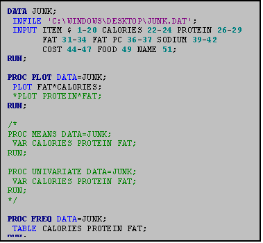These commands are illustrated in the example at the right. The asterisk (*) preceding the line which reads "PLOT PROTEIN*FAT;" will make sure that this ONE LINE is not read when the SAS program is submitted. A SECTION can be taken out by placing a forward slash followed by an asterisk (/*) at the beginning of the section and reversing these symbols at the end of the section (*/). In this example, both the PROC MEANS and PROC UNIVARIATE commands will be ignored when the program is run. The program begins again with PROC FREQ.

ø A note for those transitioning from the mainframe version of SAS: Do NOT use the ENDSAS; command unless you wish to quit the SAS System altogether. This command closes all your active windows and shuts down the program.

4.0 A CONDENSED GUIDE TO THE COLORS OF THE ENHANCED EDITOR

As mentioned throughout this manual, one big advantage of the PC SAS System is the automatic color coding that the Enhanced Editor. The statistics students who came before you spent countless hours debugging their SAS programs. The color coding will alert you immediately when some of the more common SAS programming errors occur (this is not to say that all of your programs will work on the first try…they won’t! But you will avoid many of the more frustrating errors that plagued your colleagues.) Below is table of color codes along with a sample program.

COLOR	COMMAND TYPE	EXAMPLE
BOLD BLUE	Major SAS commands	DATA
ROYAL BLUE	Sub commands, and recognized SAS words	INFILE STUDENT
PURPLE	Words within quotes such as filenames or titles.	‘C:\My Documents\DATA.DAT’
BOLD GREEN	Numbers	1-20
GREEN	Commented out commands	*PLOT;
RED	Errors	TALBE
CALORIES	All user defined words such as variable names	CALORIES RESDAT1

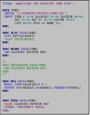The program to the right illustrates the various colors as well as 3 very common SAS errors.

First, notice that the Major SAS commands are in bold blue and the sub commands and SAS words are in royal blue. If these commands were not in these colors, we would know that we had made a mistake. For example, in the last procedure, the sub command TITLE2 appears in black. Upon closer inspection, we realize that the semi-colon has been left off the preceding command.

Also, all of the titles and file names are in purple. A common mistake occurs when the programmer forgets to close the quotation marks around a title. This is what has happened in that same TITLE command in the last procedure. The RUN; command is now in purple, because leaving off the second quotation mark has caused SAS to consider it part of the title. If a command appears in purple unexpectedly, look for a missing quotation mark.

Other errors, such as spelling errors, often appear in red. If you misspell a known SAS word or command (such as the misspelling of the sub command TABLE in the last procedure), SAS will alert you. It will NOT, however, correct you if you misspell a variable name, or other user defined word.

PART V: THE SAS LOG FILE

1.0 The Log File

Log files are your friends! While you will catch many errors with the Enhanced Editor before you submit your program, there will still be some errors that you will only find upon inspection of the LOG file. Even when you submit a program file and there are no programming errors, your LOG will contain several SAS NOTES of interest. Below is a sample SAS LOG file and some information in the right margin regarding how to interpret it.

Sample Log File Comments

1 The SAS System ª THE DATE IS INCLUDED ON

NOTE: Copyright(c) 1989 by SAS Institute Inc., Cary, NC USA. ª THIS LINE UNLESS THE NO DATE

NOTE: SAS (r) Proprietary Software Release 6.06.01 ª OPTION (OPTIONS NODATE) IS

Licensed to HARVARD UNIVERSITY GRADUATE SCHOOL OF ED., Site 0001177010.ª ADDED T0 THE PROGRAM.

ª

ª

1 OPTIONS LINESIZE=75; ª THE LINESIZE (AND NODATE)

2 title 'Junk Food Data Set Analysis'; ª OPTIONS ARE SOME OF MANY

3 ª OPTIONS YOU CAN USE IN

4 data junk; ª YOUR PROGRAM.

5 infile junk; ª

6 input item $ 1‑20 calories 22‑24 protein 26‑29 fat 31‑34 ª THIS INPUT LINE USES MORE

fat_pc 36‑37 ª THAN THE NUMBER OF

7 sodium 39‑42 cost 44‑47 food 49; ª COLUMNS SPECIFIED IN THE

8 label ITEM = 'Name of Junk Food' ª LINESIZE OPTION (75) SO IT

9 CALORIES = 'Calories per item' ª IS PRESENTED IN "WORD WRAP"

10 PROTEIN = 'Protein in Grams' ª FORM.

11 FAT = 'Fat tsp' ª

12 FAT_PC = 'Fat as percent of Calories' ª

13 SODIUM = 'Sodium in Milligrams' ª

14 COST = 'Price of Item'; ª

15 ª

ª THIS NOTE INDICATES THE

NOTE: The infile JUNK is: ª NAME OF THE RAW DATA SAS IS

File=USER1:[S030]JUNK.DAT ª READING.

ª

NOTE: 36 records were read from the infile JUNK. ª THIS NOTE INDICATES THE

The minimum record length was 51. ª FORMAT OF THE RAW DATA.

The maximum record length was 52. ª

NOTE: The data set WORK.JUNK has 36 observations and 8 variables. ª THIS NOTE TELLS YOU THAT A

ª SAS DATA FILE (WORK.JUNK)

16 PROC UNIVARIATE DATA=JUNK; ª HAS BEEN CREATED.

17 VAR COST FOOD PROTEIN; ª

18 ª

ª

NOTE: The PROCEDURE UNIVARIATE printed pages 1‑3. ª THIS NOTE TELLS YOU WHERE

ª THE PROC UNIVARIATE IS

19 PROC CORR DATA=JUNK; ª PRINTED IN THE LIS FILE.

20 VAR CALORIES FAT FAT_PC SODIUM COST; ª

21 PARTIAL PROTEIN; ª

22 ª

NOTE: The PROCEDURE CORR printed pages 4‑5. ª THIS NOTE TELLS YOU WHERE

ª THE PROC CORR IS PRINTED

23 PROC PLOT DATA=JUNK HPERCENT=50; ª IN THE LIS FILE.

24 PLOT COST*CALORIES; ª

25 PLOT COST*PROTEIN; ª

26 ª

ª

NOTE: The PROCEDURE PLOT printed page 6. ª THIS NOTE TELLS YOU WHERE

ª THE PROC PLOT IS PRINTED

27 PROC REG; ª IN THE LIS FILE.

28 MODEL COST=CALORIES; ª

NOTE: 36 observations read. ª IF THERE WERE MISSING VALUES

36 observations used in computations. ª IN PROC REG THEY WOULD BE

NOTE: The PROCEDURE REG printed page 7. ª NOTED HERE.

NOTE: SAS Institute Inc., SAS Circle, PO Box 8000, Cary, NC 27512‑8000 ª THE PROC REG IS PRINTED IN

ª THE LIS FILE.

When you submit a program and there are programming errors, the LOG file will help you determine the nature of those errors, where those errors are located, and what SAS had expected given what you programmed. The chart below illustrates some common programming errors, the type of SAS error messages you will receive when SAS detects a given error, and how to correct a given error.

1.1 Errors

Common SAS Programming Errors:

1a. No semicolon at the end of a statement

1b. Missing quote marks on titles

2. Misspelling a variable name, PROC, etc.

3. Neglecting to sort data prior to using a BY statement

4. Creating variables in a PROC statement instead of a DATA step

5. Ambiguous IF/THEN statement

6. Path to the physical data file (INFILE command) is incorrect

7. Using the letter 'o' when you mean the number 0 (zero); or using

the number 0 (zero) when you mean the letter 'O.'

All programmers, experienced and inexperienced, make errors. Do not be dismayed. Debugging (finding the errors and correcting them) takes time and patience. Often another set of eyes helps. Ask someone in your class or a Teaching Fellow to review your code. Above all else, keep calm. In this section, we review the most common mistakes and provide a checklist of things to watch out for.

When SAS detects a programming error you will receive a somewhat cryptic error message in your LOG file. The error message includes:

· the SAS error number

· message explaining the error

· the location of the error

Each type of programming error has a number. The number of the error will be listed in the error message. For the most part, knowing the error number will not be very helpful to you. If you would like, however, you can look up the error in the SAS manual. The manual provides more information about each type of error.

When SAS detects an error it provides an error message at the end of the SAS step associated with a given error. Contained in the LOG file is a printout of your SAS program file. When SAS detects an error, it underlines the error on your program. Note that the numbers next to each line of your program correspond to the line number of your program.

The next two pages present some common programming errors and approaches to handling them.

APPENDIX: CORE SYNTAX FOR 5 BASIC SAS PROCEDURES

PROC PRINT; Prints a data listing

VAR Y X1 X2 X3;

PROC UNIVARIATE PLOT FREQ; Produces univariate statistics for variable X.

VAR X; Extreme observations are noted with the NAME identifier.

ID NAME;

PROC PLOT;

PLOT Y*X; Produces a scatterplot of Y versus X.

PLOT Y*X=NAME; Uses the first letter of NAME to identify data points.

PROC CORR; Estimates Pearson correlation coefficients among Y and

VAR Y X1 X2 X3; X1, X2, and X3.

PROC REG: Fits a multiple regression model predicting Y using three

MODEL Y=X1 X2 X3; predictors--X1, X2, and X3.